Sallen-Key Filter Design Using Simulated Annealing Optimization

Code can be found here: github.com/KevinNJ

Overview:

Sallen-Key filters are useful to design because they produce a second order filter response with a really small number of readily available components. Often times the low order of the filter is a good trade-off for the number of parts required. For example, I’ve used these filters to turn a PWM signal on a micro-controller into a smooth DAC. For systems that don’t require a high bandwidth, this technique works quite well.

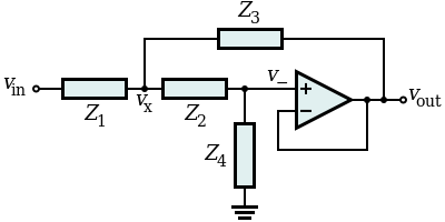
Generic circuit diagram of a Sallen-Key filter (Wikipedia)

 

Designing one of these filters is pretty easy as well, as the basic equations necessary are all available on Wikipedia – Sallen-Key topology. However, as there are two parameters and four unknowns, we have to make some arbitrary choices in the design. Usually this isn’t hard to do, but it requires some experience to find a combination of components that will meet the design criteria and perform well in real life.

Or… We could let a computer do the work for us. This lets us be lazy, and is much cooler. Richard J. Wagner from the University of Michigan wrote a wonderful little simulated annealing optimization library called PythonAnneal, which we can use to choose our part values for us.

Filter Design:

For this exercise, we’re going to design a low pass filter. The method for designing any other filter type – high pass, band pass are practically the same. I don’t see equations on Wikipedia for a notch type filter, but I’m sure they exist somewhere as well. Below is the configuration of components which make up our generic low pass filter.

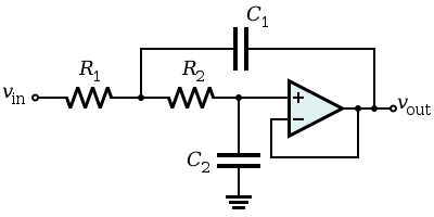
Sallen-Key low pass filter configuration (Wikipedia)

According to the schematic, we need to pick two resistor values and two capacitor values. Our goal is to pick specific components to fill in this configuration to fulfill the following:

• the filter response meets our design requirements
• the filter performs well in real life (we should avoid components that are wildly different in value, e.g. choosing 0.1 ohm  and a 1M ohm resistors.
• we have the components we choose in stock (or they are easy to get). We should avoid odd component values.

Lets assume we are trying to make a DAC with a PWM signal with a fundamental frequency of 500 Hz. We want the fundamental frequency of the PWM signal and anything above to be completely wiped out. We also want a unity response in the pass-band, or our filter will warp our desired signal. Lets set our filter criteria as follows:

• An attenuation of -40 dB at 500 Hz
• A target Q value of (maximally flat response, or no resonance peak)

Choosing -40 dB puts our fundamental frequency well below the noise floor. A nice aspect of using an optimizer is that we can set any target attenuation for any frequency. Normally, our design equations would only let us pick the natural frequency of the filter (frequency where the filter’s resonance peak happens).

Simulated Annealing:

In Simulated Annealing (SA), the computer takes a system and makes a small random change to it. The algorithm then decides if it should keep the new system or revert back to the original. With enough of these random steps, the computer finds a system which meets the optimization criteria. The full simulated annealing algorithm is slightly more complicated than this, but I’ll discuss that more in a separate post.

In order to interface with Richard’s Simulated Annealing code, we need to define two functions, which are:

• move(system)
• energy(system)

The ‘move’ function describes how to make a random change to our system. We’ll have it pick one of the four components to change, and then randomly pick a component value out of our stock to change it to.

def move(system):
    """ Changes the system randomly

    This function makes a random change to one of the component values
    in the system.
    """
    component = random.randrange(0, 4)

    if component == 0:
        index = random.randrange(0, len(cvalues))
        system[0] = cvalues[index]
    elif component == 1:
        index = random.randrange(0, len(cvalues))
        system[1] = cvalues[index]
    elif component == 2:
        index = random.randrange(0, len(rvalues))
        system[2] = rvalues[index]
    elif component == 3:
        index = random.randrange(0, len(rvalues))
        system[3] = rvalues[index]

The ‘energy’ function is a metric of how ‘good’ the current system is. In keeping in the analogy of annealing, lower energies are better than higher ones. The easiest way is to make the energy function is to start with an energy of 0 and penalize the system for each thing wrong by adding to the energy value.

target_q = 0.707
target_freq = 500
target_atten = -40

def energy(system):
    """Computes the energy of a given system.

    The energy is defined as decreasing towards zero as the system
    approaches an ideal system.
    """

    frf_ = frf(system)
    f0_ = f0(system)
    q_ = q(system)
    c1,c2,r1,r2 = system

    e = 0
    e += abs(target_atten - dB(frf_(target_freq))) / abs(target_atten) # percent error off frequency @ attenuation
    e += abs(target_q - q_) / abs(target_q)                            # percent error off ideal Q value
    e += abs(c1-c2) / abs((c1+c2)/2) * 0.1                             # percent difference in capacitor values
    e += abs(r1-r2) / abs((r1+r2)/2) * 0.1                             # percent difference in resistor values

    return e

Note how all of the energy penalties are calculated as percent differences. This helps to normalize the error against the wide differences in magnitude of the things we are comparing. For example, the target Q value is 0.707… and the target attenuation is -40. If our current system has an attenuation of -35, but the current Q is 0.2 we should be working on getting a better Q value before trying to change the attenuation. However the difference between 0.707 and 0.2 is much less than the difference between -35 and -4o. If we look at the percent difference instead, the Q adds significantly more error than the attenuation, which is what we want.

Results:

We are now ready to pop this code into PythonAnneal and see how the code does. Remember that our critera was as follows:

• An attenuation of -40 dB at 500 Hz
• A target Q value of

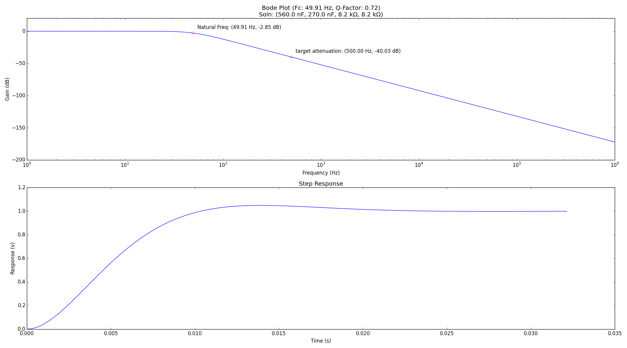
Result of Simulated Annealing Sallen-Key Design

The chosen part values can be seen in the title of the plot. They are as follows:

• C1: 560 nF
• C2: 270 nF
• R1: 8.2 kΩ
• R2: 8.2 kΩ

These are perfectly reasonable values to choose. What’s more, the Q-Factor is within 1 hundredth of the desired factor, and our target frequency shows almost exactly our desired attenuation of -40 dB. Not bad at all.

From the graph, we can see that we expect to get about 50 Hz of bandwidth from the system we designed.  This is a perfectly fine amount for controlling some physical device like a valve or whatever.  If we wanted to drive a speaker, we probably would have had to choose a higher order filter topology to reduce the space between our target frequency of 500 Hz at -40 dB and our pass band.  We would also have probably had to start with a PWM signal with a greater fundamental than 500 Hz as well…

The bottom plot shows the step response of the filter in seconds. This is useful for looking at our slew rate, or the maximum speed at which the DAC output voltage can change.