Analysis of a Weinberg Converter for Solar Panel Maximum Peak Power Tracking

LTSPICE files available here: github.com/KevinNJ.

Overview

Recently, a friend of mine has been working on a circuit for maximum power point tracking (mppt) of his solar panel array.  The circuit he’s chosen is a Weinberg DC-DC isolating buck converter, chosen for it’s very high potential efficiency.  The circuit looks pretty simple in principal, but when he built a prototype of the circuit we were seeing some effects that I didn’t understand.  I decided to simulate the circuit in SPICE, and post the results of the analysis here.

Circuit

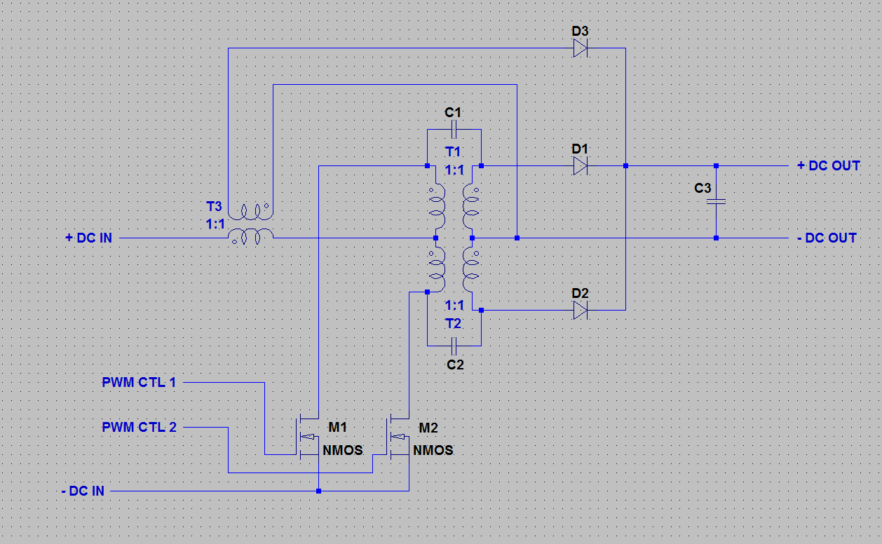
First, let’s take a look at the schematic.

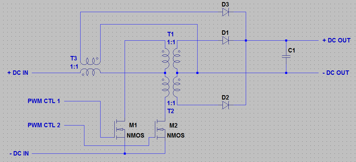
Weinberg Buck Converter

There aren’t any values chosen for this circuit, although like a lot of power circuits, I don’t think that the values of the majority of components are particularly critical – as long as all parts can handle expected voltages and currents.  Here are things to watch out for when picking parts:

• None of the transformers should not saturate when storing energy.  This has to do with the transformer core material, inductance of the primary (number of windings on the core), and switching frequency.
• Fast diodes (low voltage drop) are critical for efficiency
• Low series resistance on the inductors and ESR on the capacitors is also important for efficiency

Looking at this circuit, it’s pretty clear how it’s supposed to work.  M1 and M2 are switched on and off 180 out of phase with one another.  The duty cycle of the switching signal controls the output bus voltage.

This configuration looks a lot like two flyback converters (wikipedia) in parallel. The wikipedia article above has a good description of how this circuit works, but I’ll copy a little bit of info here for reference.

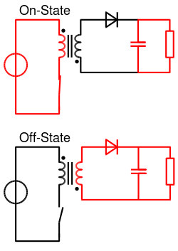
Two operating states of a flyback converter (wikipedia)

When the switch is turned on, current is drawn through the transformer, increasing the magnetic flux of the transformer core.  The voltage across the secondary is negative, reverse biasing the diode.  Energy is stored in the transformer in the form of magnetic flux.  During this half of the cycle, the load is powered from the capacitor.

When the switch is turned off, the voltage in the secondary turns positive forward biasing the diode.  The stored energy in the transformer is released through the secondary to charge the capacitor and power the load.

It looks like when either M1 or M2 are on and charging T1 or T2, a voltage is also induced across T3 charging it.  We would guess then that T3 would only discharge when both M1 and M2 are off.

Below is a table of the different states that M1 and M2 can be in against the different states that each transformer will be in.

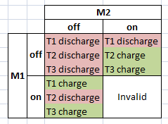
N-FET conduction vs Transformer State

And a waveform showing 1 PWM cycle of M1 and M2 against the transformer states.

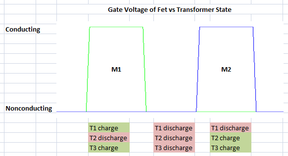
N-FET Gate Voltage vs Transformer State

Circuit Simulation and Analysis

Alright, let’s set up SPICE to handle our circuit particulars.  I’m using the following circuit:

Weinberg SPICE Model

A few quick notes about transformers in LTSPICE:

• K statements are used to make transformers from 2 inductor elements.  What will be referred to in this article as transformer T1 is marked in the SPICE schematic as K1.  T2 and T3 are marked likewise.
• In SPICE there is no such thing as a turns ratio.  The model only knows about the ratio of the inductance of each side.  To calculate the necessary inductance ratio to achive a proper turns ratio, it is helpful to remember that inductance is proportional to the square of the number of turns.
• Note that in the simulation both the primary and secondary need to be referenced to the same ground.  This guarantees that the circuit has appropriate boundary conditions and we don’t get convergence errors.  This does not need to be the case in real life.
• See Using Transformers in LTSPICE for more information.

First off, let’s look at what happens to the voltage and current on the output bus using the transient simulation.  I’ve set an end time of 15 ms which runs reasonably fast on the computer and allows the circuit to reach steady state.  The PWM inputs are set to a 25% duty cycle.

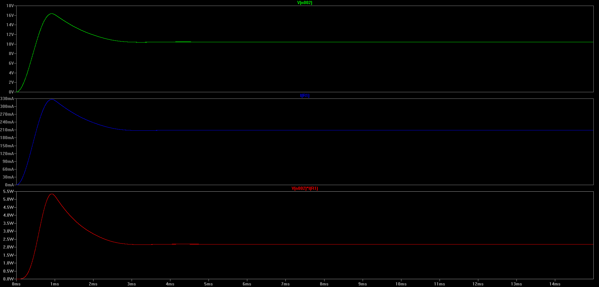
Voltage across load, current through load, and power sinked by load
(Click for higher resolution version)

So it looks like our circuit might be simulating correctly.  We appear to be generating a voltage across the load which is about 1/4 of the input voltage.  There is a transient in the first 3 ms or so which then dies out and the circuit reaches a steady state value.

Let’s see if charging and discharing of the transformers works like we think it does.  Below is the power flowing through the primary and secondary of T1.

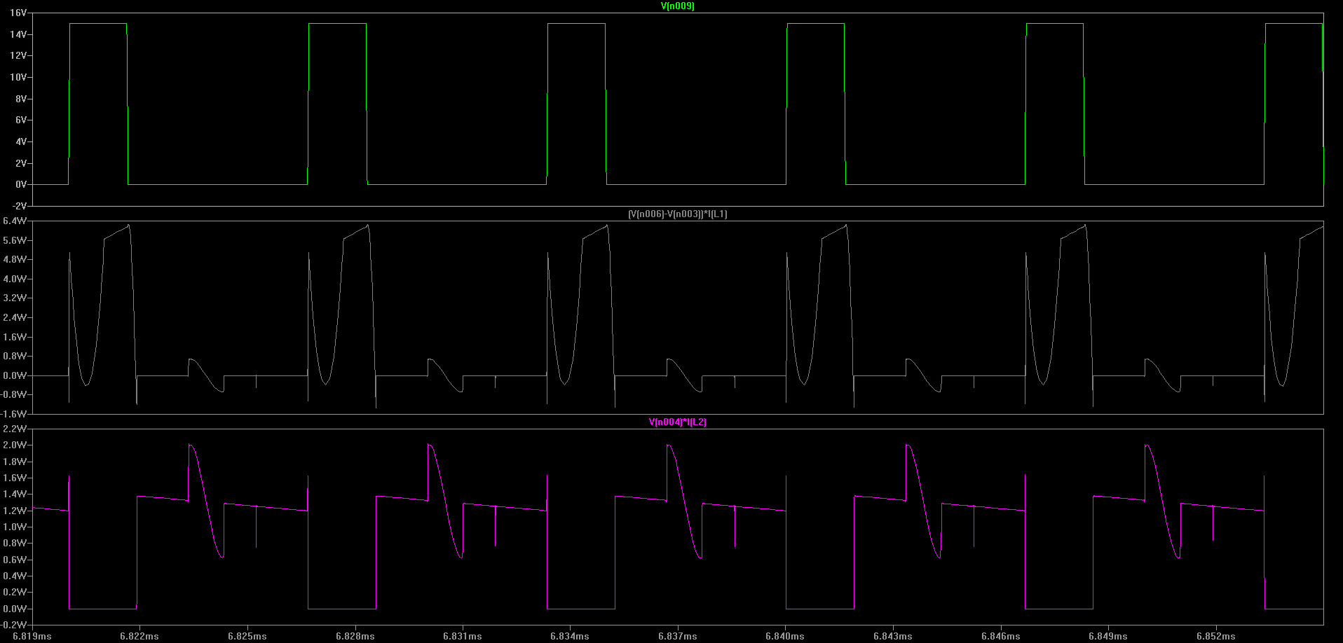
Top: Voltage applied to N-FET gate (high => FET is conducting)
 Middle: Power being sinked by T1 (K1) primary from Source
Bottom: Power being sourced by T1 (K1) secondary to Load
(Click for higher resolution version)

It looks like the system sort of works like how we guessed.  When the N-FET is on, power is stored in the T1 transformer.  When the fet is turned off, that power is sourced into the load through the secondary.  There are some ripples which haven’t been explained yet, but we can safely ignore those for now.

T2 acts identically to T1, but 180 degrees out of phase.  I’m not going to display the graphs here though to save space.

Let’s check out how the power transfer in T3 works.

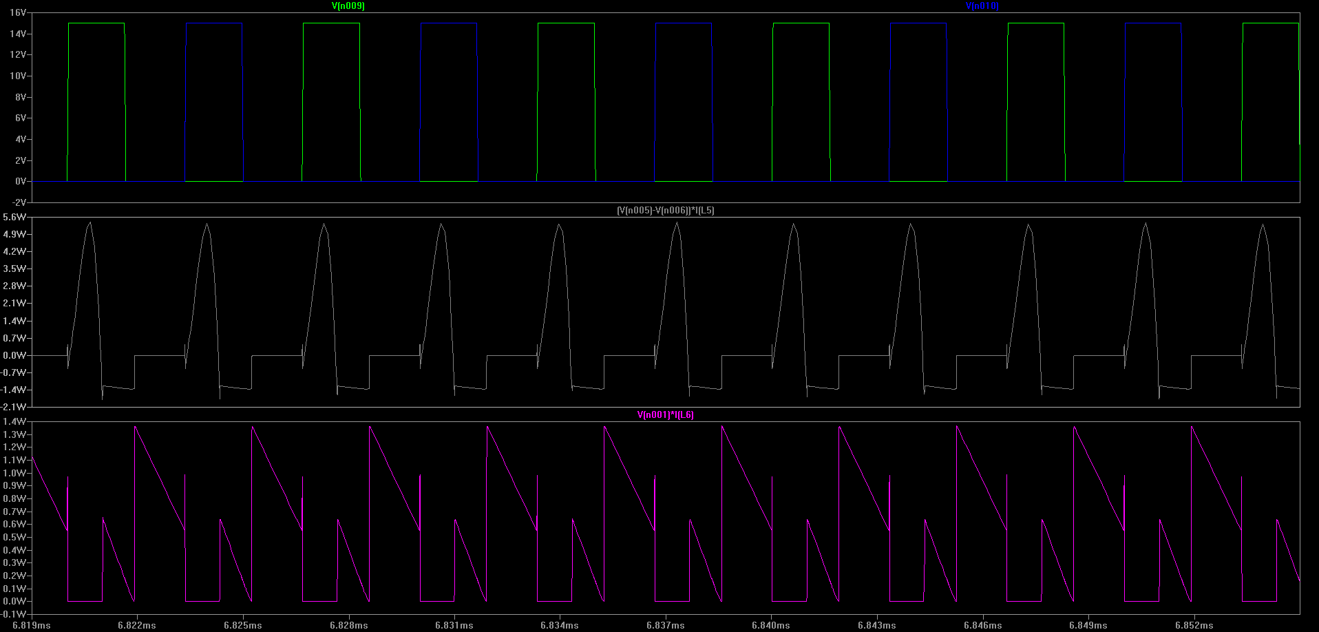
Top: Gate voltages applied to M1 (green) and M2 (blue)
Middle: Power sinked by primary of T3 (K3) from Source
Bottom: Power sourced by secondary of T3 (K3) to Load
(Click for higher resolution version)

So, every time a FET is turned on, T3 charges.  Any time that both FETs are off T3 is discharging.  So this transformer works a lot like how we guessed it would.

Unfortunately it’s a little difficult to measure power in a real circuit, so here’s a graph of the expected voltages at various places in the circuit.  This should give us expected values to look for when probing the circuit with an oscilloscope.

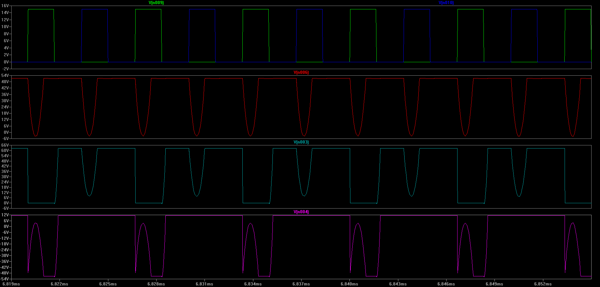
First: Voltage being applied to gates of M1 (green) and M2 (blue)
Second: Voltage between primary of T3 and T1/T2
Third: Voltage between primary of T1 and M1 N-FET
Last: Voltage between secondary of T1 and D1
(Click for higher resolution version)

After prototyping one of these circuits, it’s apparent that the actual waveforms are much less nice than these.  There are all sorts of voltage spikes and ringing which this simulation does not show.  This is most likely because we are simulating ideal inductors (coupling coefficient of 1).  It’s actually handy to do so for now because it gives us a good general picture of how we should expect the timing of events in our circuit to behave.

Leakage Inductance

The biggest problem for us in this circuit is the leakage inductance on our transformers.  Leakage inductance is caused when magnetic flux in one of the wingdings does not pass through the other winding.  It’s sort of like having an extra inductor on the end of the transformer.

Having leakage inductance causes major problems in a flyback circuit.  I don’t have a good reference which completly describe the effects of leakage inductance, but it appears that it causes the following effects in a flyback circuit:

• Significantly increased voltage transients on the MOSFETs
• High Frequency Ringing

Some references online talked about how leakage inductance affects the power transfer between the primary and the secondary.  Basically it traps some of the power in the primary causing the ringing and transients.  At first glance this seems sort of reasonable – the leakage inductance would certainly store some energy and it wouldn’t be possible for that energy to cross to the secondary.  However, I haven’t played with the circuit in SPICE enough to fully understand this effect.

Because of this, in a standard flyback circuit design, it is imperative to use tightly coupled transformers.  My guess is that torroidal or E-core transformers are the best choice – a transformer should be used where the entire flux path is made of a magnetically conductive material.

Simulating a Non-Ideal Circuit

In SPICE we can simulate the leakage inductance in our transformers.  I don’t have a good feel for the actual coupling coefficient in the real circuit we prototyped, but choosing a nice round 90% produces a more realistic simulation.

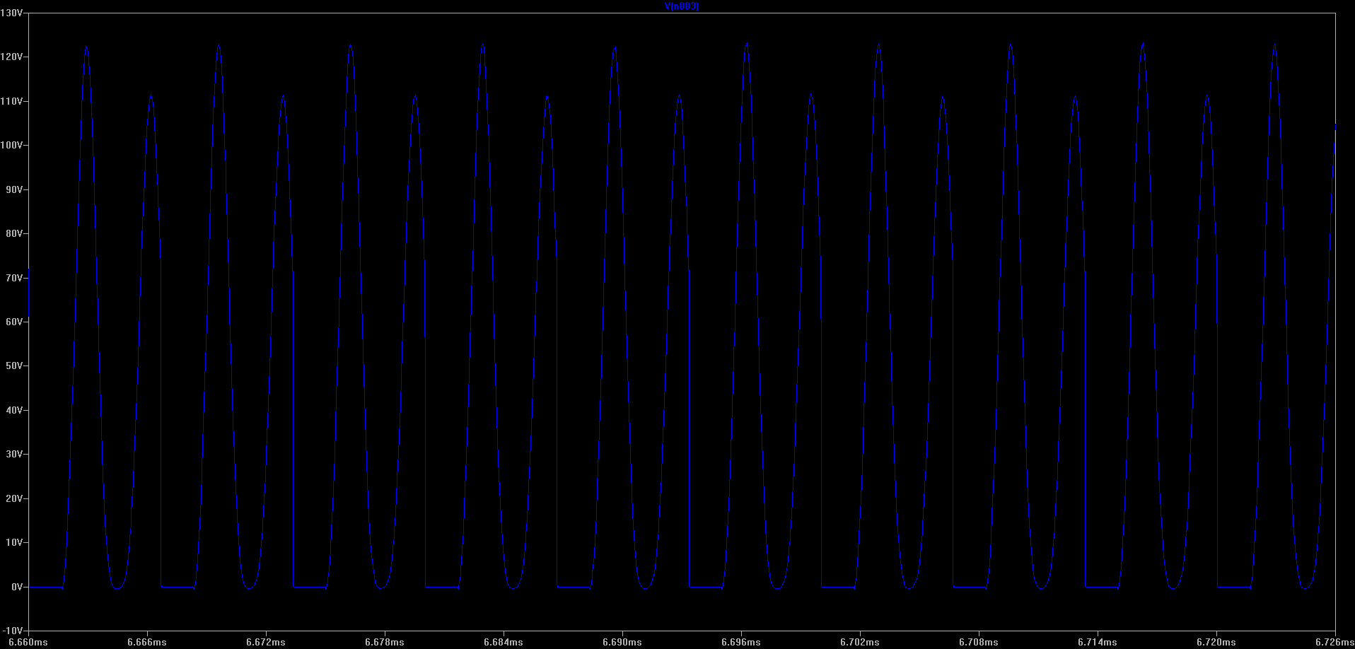
Voltage across M1 N-FET when leakage inductance has been changed to 0.9
(Click for higher resolution version)

The voltage across the N-FET basically doubled in the circuit.  This means that in the current circuit, the FETs we choose would require a very high breakdown voltage.

In the prototyped circuit we were able to push the voltage transients up past 300V before our FETs started smoking.  As it’s hard to source FETs with this kind of breakdown voltage (cheaply), some modification to the solution is required.

Snubbing the Transient Voltages

There is an interesting solution to this problem which I found when doing some background reading on flyback circuits.  The topology is called a single-ended primary inductor converter or SEPIC.

There are many different slight variations on this topology but the basic modification is to couple the primary and secondary of the inductors through a capacitor.  This helps clamp the transient voltages and remove the ringing from the circuit.

SEPIC circuit (flyback with coupling capacitors added)

Upsides of this circuit are much lower break down voltage requirements on the FETs.  This circuit is also supposed to act like a (non-inverting) buck-boost topology, although I haven’t tried simulating a condition where it boosts the voltage yet.

Downsides to this topology is the fact that the topology is 4th order making it more difficult to control.  However, I don’t think that this will be an issue in the intended use case.

Simulation of SEPIC Modifications

Setting the new capacitors to the values given below seemed to produce reasonable results.

• C1: 1 uF
• C2: 1 uF

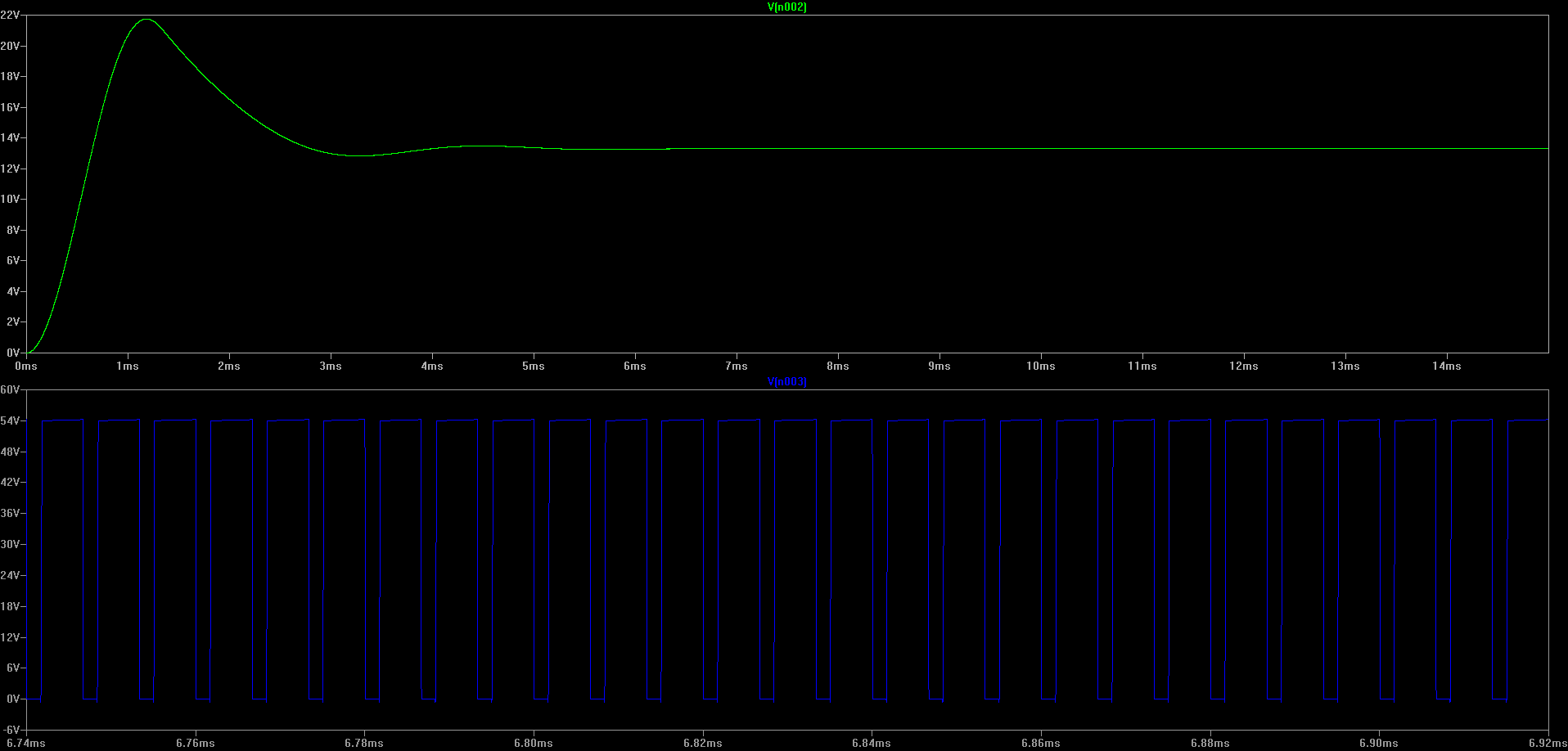
Top: Voltage on output bus
Bottom: Voltage across M1 N-FET
Note: Plots not to same time scale. (Click for higher resolution version)

From the extra ringing in the output bus, it’s evident that we’ve increased the order of the circuit.

However, when we look at the voltages across the N-FETs, the results look way more reasonable.  We’ve brought the voltage values back down basically the values on the ideal circuit!  Also, the ringing we were seeing seems to completely have disappeared.

Related Reading

• Power Tip 32: Beware of circulating currents in a SEPIC coupled-inductor–Part 1
• AN-1484 Designing A SEPIC Converter
• Using Transformers in LTspice/SwitcherCAD III
• Measuring Leakage Inductance

Decision Trees in Python

Code available here: github.com/KevinNJ

Overview:

So, I was trying to solve XKCD’s infinite resistor problem (xkcd.com/356). After some thought, this method probably won’t be useful, but it still has some interesting applications.

 Problem:

On a infinite grid, find all paths which connect two given points.

The only rule for movement is that you may not move immediately back the way you came. For clarification, the movements happen on the lines of the grid – from the point where you stand, you may move left, right, up or down. There are no diagonal movements.

Infinite 2D grid

For instance, if you had just moved from left to right, then the valid move for the next turn are up, down, and right.

Valid Moves

The problem is to find all possible paths of length N which will take you from point A to point B.

Counting the Shortest Paths:

The first important observation to make is that the shortest path from A to B is 3 units long and involves 2 decisions to move right, and one decision to move up. It does not matter what order these decisions are made in.

With just this information, we can determine how many paths of length 3 exist using the binomial theorem. There are 3 choices of 2 possibilities, and 2 of those choices must be left. Or equivalently, there are 3 choices of 2 possibilities, and 1 of those choices must be up.

This counting method works for any two points on a grid of any distance apart.

Finding the Shortest Paths:

When there are decisions to be made, we can use a decision tree to help us find all possible results. We can make a recursive algorithm to build this tree which is pretty straightforward.

• Start with a tuple representing the decisions you can make. E.g (0L, 2R, 1U, 0D)
• For each action that we could take:
  • Make a child node, and label it with our decision
  • Subtract that decision from our tuple
  • Recursively call our function on this child node with the new tuple

The algorithm terminates when there are no more actions which we can take because the child tuple contains all zeros in any of the move directions we are allowed to go.

Here’s the code in python:

transitions = {
    'L': ['U', 'D', 'L'],
    'R': ['U', 'D', 'R'],
    'U': ['L', 'R', 'U'],
    'D': ['L', 'R', 'D'],
    None: ['L', 'R', 'U', 'D']
}

class Node(object):
    def __init__(self):
        self.children = []
        self.decision = None

def make_tree(node, state):
    """Make our decision tree

    state is a dictionary containing four keys, which are
    L,R,U,D
    """
    for d,v in state.iteritems():
        if d in transitions[node.decision] and v > 0:
            child = Node()
            child.decision = d
            new_state = state.copy()
            new_state[d] -= 1
            make_tree(child, new_state)
            node.children.append(child)

def run_tuple(tup):
    root = Node()
    l,r,u,d = tup   # unpack decisions
    make_tree(root, {'L':l, 'R':r, 'U':u, 'D':d})

    return root    # return the tree we just made

 Finding Longer Paths:

To find other paths, we only need to make the observation that we must always add decisions to our tuple in pairs – if we make an extra left, then at some point we must make another right, and the same with up and down.

Because we must always add decisions in pairs, longer paths will always have the same parity as the shortest possible path. So in this case, because the shortest path is of length 3, we can only make paths with an odd length (5, 7, 9, etc).

For example, here are tuples for paths of length 3, 5, and 7.

#(L, R, U, D)

 (0, 2, 1, 0)  # length 3 (base decisions)
 (1, 3, 1, 0)  # length 5 (add 1 to L,R)
 (0, 2, 2, 1)  # length 5 (add 1 to U,D)
 (1, 3, 2, 1)  # length 7 (add 1 to L,R  add 1 to L,D)
 (2, 4, 1, 0)  # length 7 (add 2 to L,r)
 (0, 2, 3, 2)  # length 7 (add 2 to U,D)

Notice that the length of the path is equivalent to the number of decisions to be made. That is, if we add up the numbers in the tuple, we come out with the path length.

Visualizing the Trees:

Now we’ve made our trees, but they aren’t really useful if we can’t extract information from them.  Fortunately, there’s a handy program called GraphViz with a python API called pydot which we can use to make pictures of our trees.

Here’s our algorithm:

• For each child in the node we were passed
  • Make a new child node in the GraphViz graph
  • Label it with our move direction decision
  • Connected the new GraphViz child node to our current node
  • Call recursively on the child node

# Note that root, and child our nodes in our tree
# gv_root and gv_child are the GraphViz objects

def make_graph(gv_graph, root, gv_root):
    for child in root.children:
        gv_child = pydot.Node(get_next_id(), label=child.decision)
        gv_edge = pydot.Edge(gv_root, gv_child)
        gv_graph.add_node(gv_child)
        gv_graph.add_edge(gv_edge)
        make_graph(gv_graph, child, gv_child)

We start with a root node labeled with an X representing the fact that at this node, we haven’t made a decision yet.

# make our decision tree from our tuple of possible decisions
root = run_tuple((0,2,1,0))

# save our graph as a picture so that we can look at it
gv_graph = pydot.Dot(graph_type='graph', dpi=300)
gv_root = pydot.Node('X')
make_graph(gv_graph, root, root_node)
gv_graph.write_png('graph.png')

Results:

Path length 3, decison tuple (L0, R2, U1, D0)

(L0,R2,U1,D0) Length:3

Notice that our algorithm finds all 3 paths.  In our decision tree, the number of paths, is equivalent to the number of leaf nodes.

The way to read this tree is pretty simple.

• Put your finger on point A on the grid.
• Start at the X on the tree.
• Choose a child to move to (R or U)
• Move your finger right, or up, depending on your choice
• Repeat until you reach the bottom of the tree

Lets look at a longer path – how about length 5, (L1, R3, U1, D0).

(L1, R3, U1, D0) Length: 5

Hang on, some of these paths aren’t long enough.  In fact only 2 paths in the tree are of length 5.  With some introspection this makes sense – the algorithm terminates when all possible moves are expired.  With our move rules, it is certainly possible to trap yourself so that the only move you are allowed is back the way you came, in which case the algorithm terminates.

So, really we should cull any paths from the tree which are not of the length path which we are looking for.

Applications:

When I went about writing this code, I was hoping to visualize the XKCD resistor grid problem as parallel paths of resistance equal to the path length.  Being able to count the paths would make building a closed form for the resistance pretty easy.

After writing the code and thinking about it, I realized that this method was not a good model for electricity – for instance flowing electricity would never make loops in the grid which this method does not disallow.

Still, this is an interesting twist on the path finding through a grid, so I thought it might be interesting to post.

Short Time Fourier Transform using Python and Numpy

Code available here: github.com/KevinNJ

Overview:

The Short Time Fourier Transform (STFT) is a special flavor of a Fourier transform where you can see how your frequencies in your signal change through time.  It works by slicing up your signal into many small segments and taking the fourier transform of each of these.  The result is usually a waterfall plot which shows frequency against time.  I’ll talk more in depth about the STFT in a later post, for now let’s focus on the code.

I was looking for a way to do STFT’s using Numpy, but to my chagrin it looks like there isn’t an easy function implemented.  Well then, I’ll just write my own.

Goal:

First, let’s look at the desired result that I’m trying to obtain. Here is a spectrum of a whistle performed by my friend Mike.

Spectrum of a whistle

You can see that there is a strong frequency around 2200 Hz which makes this note about a C# or Dd in the 7th octave.  Mike  The second harmonic is also fairly strong at 4400 Hz.

Here is a picture of a whistle which increases in frequency over time.

Spectrum of a chirp like whistle

It goes from 880 Hz (A in the 5th octave) all the way up to 1760 Hz (A in the 6th octave).  I find it remarkable how precisely Mike managed to whistle an octave as he wasn’t trying to do that…

 STFT Algorithm:

So, we understand what we’re trying to make – now we have to figure out how to make it.  The data flow we have to achieve is pretty simple, as we only need to do the following steps:

1. Pick out a short segment of data from the overall signal
2. Multiply that segment against a half-cosine function
3. Pad the end of the segment with zeros
4. Take the Fourier transform of that segment and normalize it into positive and negative frequencies
5. Combine the energy from the positive and negative frequencies together, and display the one-sided spectrum
6. Scale the resulting spectrum into dB for easier viewing
7. Clip the signal to remove noise past the noise floor which we don’t care about

Step 1 – Pick segment: We need to find our current segment to process from the overall data set.  We use the concept of a ‘sliding window’ to help us visualize what’s happening.  The data inside the window is the current segment to be processed.

Sliding window on top of data

The window’s length remains the same during the processing of the data, but the offset changes with each step of the algorithm.  Usually when processing the STFT, the change in offset will be less than one window length, meaning that the last window and the current window overlap.  If we define the window size, and the percentage of overlap, we know all the information we need about how the window moves throughout the processing.

Step 2 – Multiply by half-cosine: This helps to alleviate a problem created by segmenting the data.  When the data is cut into pieces, the edges make a sharp transition that didn’t exist before.  Multiplying by a half cosine function helps to fade the signal in and out so that the transitions at the edges do not affect the Fourier transform of the data.

Data multiplied by a half cosine

There is an additional benefit to using a half cosine window.  It can be shown that with an overlap factor of 50%, the sum of the windows is a constant value of 1.  This means that multiplying our data by this particular function does not introduce differences in amplitude from the original signal.  This is mostly important if the waveform has some type of units attached to it [pascals] and we want the frequencies in the Fourier transform to correctly represent the energy content of each frequency in those units.

Half cosine windows combining into a unity gain.

Step 3 – Pad Data: We pad the end of the current segment with a number of zeros equal to the length of the window.  Or in other words, the new segment will be twice as long as the original segment.  The reason for this is explained later.

Step 4 – Fourier Transform and Scale: This is where all the magic happens.  Everything up to this point was just preparing the data, but this step is the beating heart of the algorithm.  Here we finally take the Fourier transform of the data.  I’m not going to explain the Fourier transform here except to say that it takes a signal and extracts the frequency content from that signal.  There are a few other things that need to be remembered about the Fourier transform.

• The number of samples of data in is equal to the number of frequency bins out
• The maximum frequency that can be represented is the Nyquist frequency, or half the sampling frequency of the data.
• In the the Discrete Fourier Transform (what we are using) the order of the frequency bins is 0 Hz (DC component), positive frequencies, Nyquist Frequency, negative frequencies
• The data from the Fourier transform needs to be scaled by the number of samples in the transform to maintain equal energy (according to Parseval’s theorem)

Step 5 – Autopower: This is just more post processing to make the results more palatable to look at.  We find the autopower spectrum from the results of the Fourier transform.  The autopower spectrum is a one-sided spectrum (only contains positive frequencies) as opposed to the two-sided spectrum returned by the Fourier transform – so it’s more like the actual real world which does not contain negative frequencies.  The autopower spectrum is also scaled to represent the energy content that was in both the positive and negative frequencies of the Fourier transform.  This is important for the ‘correctness’ of the energy content of each frequency, but also has the handy benefit of suppressing lower energy content and dramatizing higher energy content.  Usually people only care about the higher energy content, so finding this transform typically makes the data much easier to look at.

Part of taking the autopwer spectrum is throwing away the upper half of the array of data.  This is why we padded the segment to twice it’s size – so that when the result was cut down by half by the autopower transform, we would still have the same number of frequency bins as samples in our segment.  Note that this isn’t a strict requirement of the algorithm – to have the segment size as frequency bins.  We could have chosen our pad length to be any number from zero (no padding) to infinity.  There is a trade off here which is too heavy in theory to go into fully here, suffice to say that I found this decision works well and simplifies the math.

Step 6 – Convert to DB: This is another transform to make the data easier to look at.  It turns out that peoples ears work on a logarithmic scale so that the ear can detect much finer changes in amplitude at low amplitudes than at high amplitudes.  We transform the data into decibels (dB) which is a logarithmic scale, so that we can see the energy content of a signal more how our ears would detect it.  Converting the data to decibels has the effect of stretching peaks downwards towards the average sound level, and bringing troughs upwards.  This allows us to compare content at all amplitude levels.  If we didn’t do this and we scaled the data so that the peaks were visible, it would be impossible to see any shape in the quieter values, vs if we looked at the quieter values, the peaks would explode off the top of the screen.

Step 7 – Clip Data: This also makes the data easier to look at.  We know from experience that everything below -40 dB is well below the noise floor and is probably just numerical error in the algorithm.  Therefore, we can clip the data so that everything below -40 dB is set to -40 dB exactly.  This gives us more color range to apply to significant portions of our data.

Here’s what the code looks like:

# data = a numpy array containing the signal to be processed
# fs = a scalar which is the sampling frequency of the data

hop_size = np.int32(np.floor(fft_size * (1-overlap_fac)))
pad_end_size = fft_size          # the last segment can overlap the end of the data array by no more than one window size
total_segments = np.int32(np.ceil(len(data) / np.float32(hop_size)))
t_max = len(data) / np.float32(fs)

window = np.hanning(fft_size)  # our half cosine window
inner_pad = np.zeros(fft_size) # the zeros which will be used to double each segment size

proc = np.concatenate((data, np.zeros(pad_end_size)))              # the data to process
result = np.empty((total_segments, fft_size), dtype=np.float32)    # space to hold the result

for i in xrange(total_segments):                      # for each segment
    current_hop = hop_size * i                        # figure out the current segment offset
    segment = proc[current_hop:current_hop+fft_size]  # get the current segment
    windowed = segment * window                       # multiply by the half cosine function
    padded = np.append(windowed, inner_pad)           # add 0s to double the length of the data
    spectrum = np.fft.fft(padded) / fft_size          # take the Fourier Transform and scale by the number of samples
    autopower = np.abs(spectrum * np.conj(spectrum))  # find the autopower spectrum
    result[i, :] = autopower[:fft_size]               # append to the results array

result = 20*np.log10(result)          # scale to db
result = np.clip(result, -40, 200)    # clip values

Displaying the Data:

Once we’ve completed the processing, we need to display our results on screen.  This is pretty easy actually – the algorithm returns a 2D array of data with values ranging from -40 to our maximum value.  One axis of the array represent frequency bins, and the other represents the segment number that was processed to get the frequency data.

Using matplotlib, we can simply display this array as an image.  We’ll apply a color map so that -40 is dark blue, and our signal maximum is red and let matplotlib do all the heavy lifting to scale and interpolate our array to the size of our image, and then display it on screen.

We have to do some math to figure out what frequency each column in the array represents and what point in time each row represents, but after we have that, we can make tick marks and take a look at our data.

img = plt.imshow(result, origin='lower', cmap='jet', interpolation='nearest', aspect='auto')
plt.show()

There is more code for making the GUI shown in the images above which will be posted soon.

Sallen-Key Filter Design Using Simulated Annealing Optimization

Code can be found here: github.com/KevinNJ

Overview:

Sallen-Key filters are useful to design because they produce a second order filter response with a really small number of readily available components. Often times the low order of the filter is a good trade-off for the number of parts required. For example, I’ve used these filters to turn a PWM signal on a micro-controller into a smooth DAC. For systems that don’t require a high bandwidth, this technique works quite well.

Generic circuit diagram of a Sallen-Key filter (Wikipedia)

 

Designing one of these filters is pretty easy as well, as the basic equations necessary are all available on Wikipedia – Sallen-Key topology. However, as there are two parameters and four unknowns, we have to make some arbitrary choices in the design. Usually this isn’t hard to do, but it requires some experience to find a combination of components that will meet the design criteria and perform well in real life.

Or… We could let a computer do the work for us. This lets us be lazy, and is much cooler. Richard J. Wagner from the University of Michigan wrote a wonderful little simulated annealing optimization library called PythonAnneal, which we can use to choose our part values for us.

Filter Design:

For this exercise, we’re going to design a low pass filter. The method for designing any other filter type – high pass, band pass are practically the same. I don’t see equations on Wikipedia for a notch type filter, but I’m sure they exist somewhere as well. Below is the configuration of components which make up our generic low pass filter.

Sallen-Key low pass filter configuration (Wikipedia)

According to the schematic, we need to pick two resistor values and two capacitor values. Our goal is to pick specific components to fill in this configuration to fulfill the following:

• the filter response meets our design requirements
• the filter performs well in real life (we should avoid components that are wildly different in value, e.g. choosing 0.1 ohm  and a 1M ohm resistors.
• we have the components we choose in stock (or they are easy to get). We should avoid odd component values.

Lets assume we are trying to make a DAC with a PWM signal with a fundamental frequency of 500 Hz. We want the fundamental frequency of the PWM signal and anything above to be completely wiped out. We also want a unity response in the pass-band, or our filter will warp our desired signal. Lets set our filter criteria as follows:

• An attenuation of -40 dB at 500 Hz
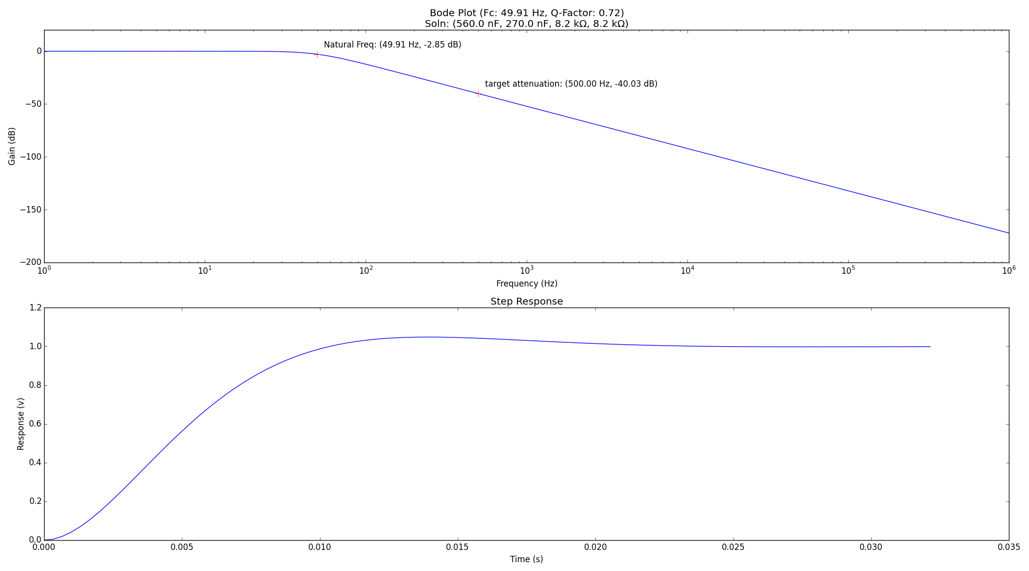
• A target Q value of (maximally flat response, or no resonance peak)

Choosing -40 dB puts our fundamental frequency well below the noise floor. A nice aspect of using an optimizer is that we can set any target attenuation for any frequency. Normally, our design equations would only let us pick the natural frequency of the filter (frequency where the filter’s resonance peak happens).

Simulated Annealing:

In Simulated Annealing (SA), the computer takes a system and makes a small random change to it. The algorithm then decides if it should keep the new system or revert back to the original. With enough of these random steps, the computer finds a system which meets the optimization criteria. The full simulated annealing algorithm is slightly more complicated than this, but I’ll discuss that more in a separate post.

In order to interface with Richard’s Simulated Annealing code, we need to define two functions, which are:

• move(system)
• energy(system)

The ‘move’ function describes how to make a random change to our system. We’ll have it pick one of the four components to change, and then randomly pick a component value out of our stock to change it to.

def move(system):
    """ Changes the system randomly

    This function makes a random change to one of the component values
    in the system.
    """
    component = random.randrange(0, 4)

    if component == 0:
        index = random.randrange(0, len(cvalues))
        system[0] = cvalues[index]
    elif component == 1:
        index = random.randrange(0, len(cvalues))
        system[1] = cvalues[index]
    elif component == 2:
        index = random.randrange(0, len(rvalues))
        system[2] = rvalues[index]
    elif component == 3:
        index = random.randrange(0, len(rvalues))
        system[3] = rvalues[index]

The ‘energy’ function is a metric of how ‘good’ the current system is. In keeping in the analogy of annealing, lower energies are better than higher ones. The easiest way is to make the energy function is to start with an energy of 0 and penalize the system for each thing wrong by adding to the energy value.

target_q = 0.707
target_freq = 500
target_atten = -40

def energy(system):
    """Computes the energy of a given system.

    The energy is defined as decreasing towards zero as the system
    approaches an ideal system.
    """

    frf_ = frf(system)
    f0_ = f0(system)
    q_ = q(system)
    c1,c2,r1,r2 = system

    e = 0
    e += abs(target_atten - dB(frf_(target_freq))) / abs(target_atten) # percent error off frequency @ attenuation
    e += abs(target_q - q_) / abs(target_q)                            # percent error off ideal Q value
    e += abs(c1-c2) / abs((c1+c2)/2) * 0.1                             # percent difference in capacitor values
    e += abs(r1-r2) / abs((r1+r2)/2) * 0.1                             # percent difference in resistor values

    return e

Note how all of the energy penalties are calculated as percent differences. This helps to normalize the error against the wide differences in magnitude of the things we are comparing. For example, the target Q value is 0.707… and the target attenuation is -40. If our current system has an attenuation of -35, but the current Q is 0.2 we should be working on getting a better Q value before trying to change the attenuation. However the difference between 0.707 and 0.2 is much less than the difference between -35 and -4o. If we look at the percent difference instead, the Q adds significantly more error than the attenuation, which is what we want.

Results:

We are now ready to pop this code into PythonAnneal and see how the code does. Remember that our critera was as follows:

• An attenuation of -40 dB at 500 Hz
• A target Q value of

Result of Simulated Annealing Sallen-Key Design

The chosen part values can be seen in the title of the plot. They are as follows:

• C1: 560 nF
• C2: 270 nF
• R1: 8.2 kΩ
• R2: 8.2 kΩ

These are perfectly reasonable values to choose. What’s more, the Q-Factor is within 1 hundredth of the desired factor, and our target frequency shows almost exactly our desired attenuation of -40 dB. Not bad at all.

From the graph, we can see that we expect to get about 50 Hz of bandwidth from the system we designed.  This is a perfectly fine amount for controlling some physical device like a valve or whatever.  If we wanted to drive a speaker, we probably would have had to choose a higher order filter topology to reduce the space between our target frequency of 500 Hz at -40 dB and our pass band.  We would also have probably had to start with a PWM signal with a greater fundamental than 500 Hz as well…

The bottom plot shows the step response of the filter in seconds. This is useful for looking at our slew rate, or the maximum speed at which the DAC output voltage can change.