Decision Trees in Python

Code available here: github.com/KevinNJ

Overview:

So, I was trying to solve XKCD’s infinite resistor problem (xkcd.com/356). After some thought, this method probably won’t be useful, but it still has some interesting applications.

 Problem:

On a infinite grid, find all paths which connect two given points.

The only rule for movement is that you may not move immediately back the way you came. For clarification, the movements happen on the lines of the grid – from the point where you stand, you may move left, right, up or down. There are no diagonal movements.

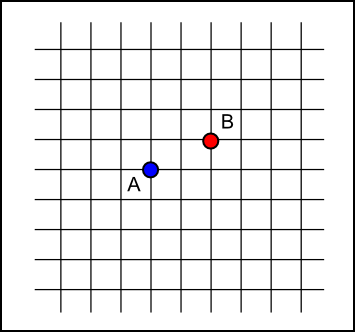
Infinite 2D grid

For instance, if you had just moved from left to right, then the valid move for the next turn are up, down, and right.

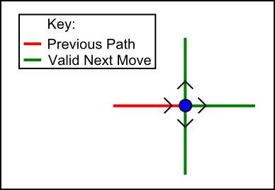
Valid Moves

The problem is to find all possible paths of length N which will take you from point A to point B.

Counting the Shortest Paths:

The first important observation to make is that the shortest path from A to B is 3 units long and involves 2 decisions to move right, and one decision to move up. It does not matter what order these decisions are made in.

With just this information, we can determine how many paths of length 3 exist using the binomial theorem. There are 3 choices of 2 possibilities, and 2 of those choices must be left. Or equivalently, there are 3 choices of 2 possibilities, and 1 of those choices must be up.

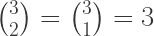
This counting method works for any two points on a grid of any distance apart.

Finding the Shortest Paths:

When there are decisions to be made, we can use a decision tree to help us find all possible results. We can make a recursive algorithm to build this tree which is pretty straightforward.

• Start with a tuple representing the decisions you can make. E.g (0L, 2R, 1U, 0D)
• For each action that we could take:
  • Make a child node, and label it with our decision
  • Subtract that decision from our tuple
  • Recursively call our function on this child node with the new tuple

The algorithm terminates when there are no more actions which we can take because the child tuple contains all zeros in any of the move directions we are allowed to go.

Here’s the code in python:

transitions = {
    'L': ['U', 'D', 'L'],
    'R': ['U', 'D', 'R'],
    'U': ['L', 'R', 'U'],
    'D': ['L', 'R', 'D'],
    None: ['L', 'R', 'U', 'D']
}

class Node(object):
    def __init__(self):
        self.children = []
        self.decision = None

def make_tree(node, state):
    """Make our decision tree

    state is a dictionary containing four keys, which are
    L,R,U,D
    """
    for d,v in state.iteritems():
        if d in transitions[node.decision] and v > 0:
            child = Node()
            child.decision = d
            new_state = state.copy()
            new_state[d] -= 1
            make_tree(child, new_state)
            node.children.append(child)

def run_tuple(tup):
    root = Node()
    l,r,u,d = tup   # unpack decisions
    make_tree(root, {'L':l, 'R':r, 'U':u, 'D':d})

    return root    # return the tree we just made

 Finding Longer Paths:

To find other paths, we only need to make the observation that we must always add decisions to our tuple in pairs – if we make an extra left, then at some point we must make another right, and the same with up and down.

Because we must always add decisions in pairs, longer paths will always have the same parity as the shortest possible path. So in this case, because the shortest path is of length 3, we can only make paths with an odd length (5, 7, 9, etc).

For example, here are tuples for paths of length 3, 5, and 7.

#(L, R, U, D)

 (0, 2, 1, 0)  # length 3 (base decisions)
 (1, 3, 1, 0)  # length 5 (add 1 to L,R)
 (0, 2, 2, 1)  # length 5 (add 1 to U,D)
 (1, 3, 2, 1)  # length 7 (add 1 to L,R  add 1 to L,D)
 (2, 4, 1, 0)  # length 7 (add 2 to L,r)
 (0, 2, 3, 2)  # length 7 (add 2 to U,D)

Notice that the length of the path is equivalent to the number of decisions to be made. That is, if we add up the numbers in the tuple, we come out with the path length.

Visualizing the Trees:

Now we’ve made our trees, but they aren’t really useful if we can’t extract information from them.  Fortunately, there’s a handy program called GraphViz with a python API called pydot which we can use to make pictures of our trees.

Here’s our algorithm:

• For each child in the node we were passed
  • Make a new child node in the GraphViz graph
  • Label it with our move direction decision
  • Connected the new GraphViz child node to our current node
  • Call recursively on the child node

# Note that root, and child our nodes in our tree
# gv_root and gv_child are the GraphViz objects

def make_graph(gv_graph, root, gv_root):
    for child in root.children:
        gv_child = pydot.Node(get_next_id(), label=child.decision)
        gv_edge = pydot.Edge(gv_root, gv_child)
        gv_graph.add_node(gv_child)
        gv_graph.add_edge(gv_edge)
        make_graph(gv_graph, child, gv_child)

We start with a root node labeled with an X representing the fact that at this node, we haven’t made a decision yet.

# make our decision tree from our tuple of possible decisions
root = run_tuple((0,2,1,0))

# save our graph as a picture so that we can look at it
gv_graph = pydot.Dot(graph_type='graph', dpi=300)
gv_root = pydot.Node('X')
make_graph(gv_graph, root, root_node)
gv_graph.write_png('graph.png')

Results:

Path length 3, decison tuple (L0, R2, U1, D0)

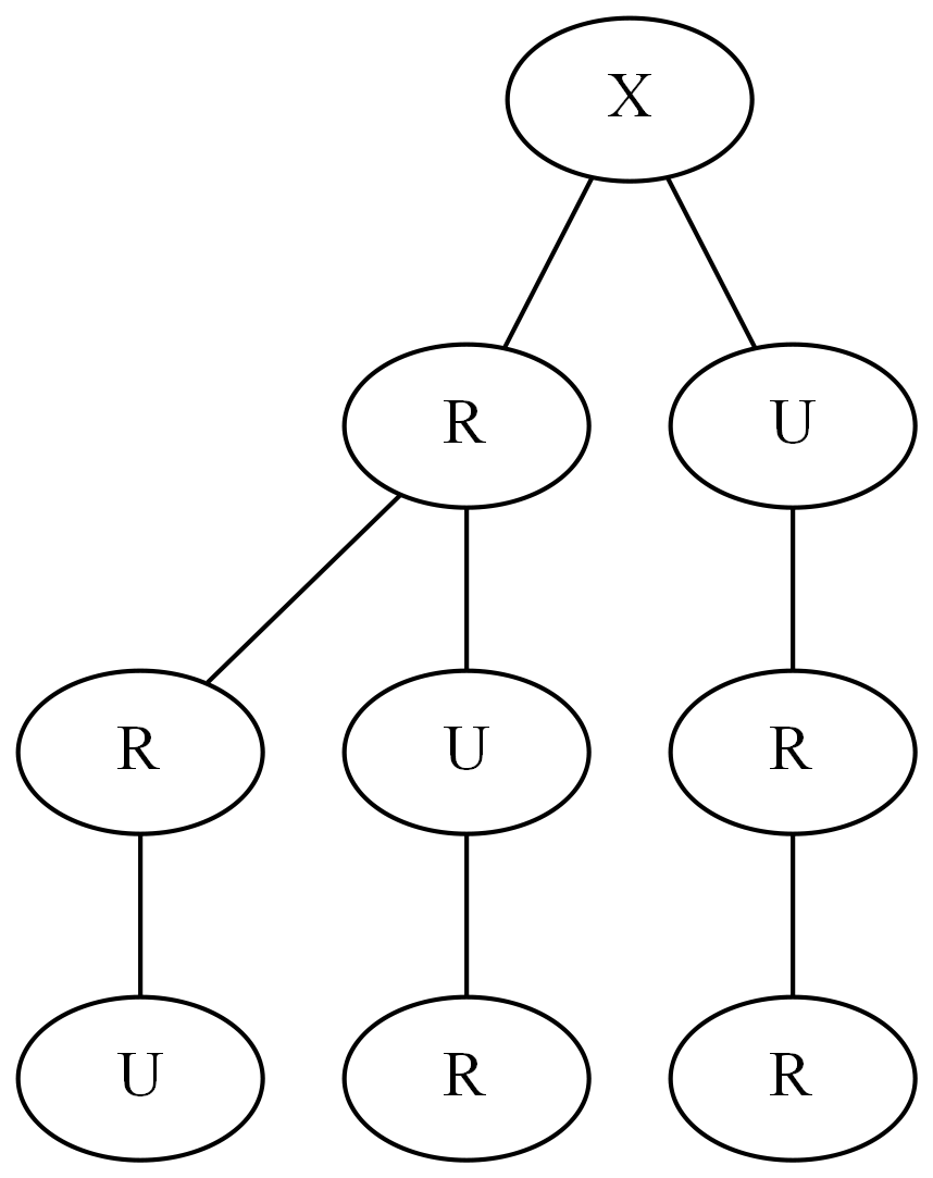
(L0,R2,U1,D0) Length:3

Notice that our algorithm finds all 3 paths.  In our decision tree, the number of paths, is equivalent to the number of leaf nodes.

The way to read this tree is pretty simple.

• Put your finger on point A on the grid.
• Start at the X on the tree.
• Choose a child to move to (R or U)
• Move your finger right, or up, depending on your choice
• Repeat until you reach the bottom of the tree

Lets look at a longer path – how about length 5, (L1, R3, U1, D0).

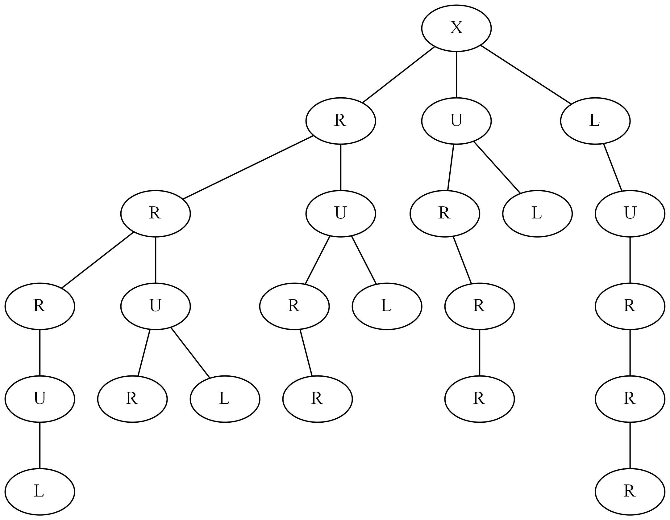
(L1, R3, U1, D0) Length: 5

Hang on, some of these paths aren’t long enough.  In fact only 2 paths in the tree are of length 5.  With some introspection this makes sense – the algorithm terminates when all possible moves are expired.  With our move rules, it is certainly possible to trap yourself so that the only move you are allowed is back the way you came, in which case the algorithm terminates.

So, really we should cull any paths from the tree which are not of the length path which we are looking for.

Applications:

When I went about writing this code, I was hoping to visualize the XKCD resistor grid problem as parallel paths of resistance equal to the path length.  Being able to count the paths would make building a closed form for the resistance pretty easy.

After writing the code and thinking about it, I realized that this method was not a good model for electricity – for instance flowing electricity would never make loops in the grid which this method does not disallow.

Still, this is an interesting twist on the path finding through a grid, so I thought it might be interesting to post.